While on the road of learning algorithmic trading, backtesting provides a safe and efficient way to examine the performance of strategies. In this article, I would like to share my experience of testing a trend following strategy through different approaches.
A smooth mean average(SMA) crossover strategy is implemented on the historical data of BTC-BUSD asset. The trading logic is when the fast line of price crossing the slow line of price from below, a buy signal is on. Vice versa, the sell signal is on when fast one crossing slow one from above. 10 day’s average price(sma10) is used as fast line, and 20 day’s average price(sma20) is for slow line.
Let’s try to achieve this strategy from basic packages. Taking advantage of Pandas.DataFrame rolling method, the values of two lines are calculated.
price_btc['close_sma10'] = price_btc['Close'].rolling(10).mean()
price_btc['close_sma20'] = price_btc['Close'].rolling(20).mean()
The signals are appeared when these two values crossing. I just assign a boolean value when sma10 is greater than sma20. This results in a column containing 0 and 1. The trading signals are located in the transition between 0 and 1 dates. These can be obtained by substracting the boolean column with its one-day shift value.
price_btc['c10_High'] = np.where(price_btc['close_sma10'] > price_btc['close_sma20'], 1, 0)
price_btc['signals'] = np.where((price_btc['c10_High'] - price_btc['c10_High'].shift(1)) == 1, 1, 0)
price_btc['signals'] = np.where((price_btc['c10_High'] - price_btc['c10_High'].shift(1)) == -1, -1, price_btc['signals'])
After getting the signals, we have to add the a boolen column to represent the status of our position. It is 1 for holding the asset. Vice versa.
position = np.zeros(price_btc.shape[0])
for i in range(price_btc.shape[0]):
    if price_btc['signals'][i] == 1:
        position[i:] += 1
    if (price_btc['signals'][i] == -1) & (position[i] == 1):
        position[i:] -= 1
To calculate the cumulative return, it is simply multiplying the daily return with the corresponding position.
price_btc['return'] = price_btc['Close'].pct_change()
price_btc['position'] = pd.Series(position, index=price_btc.index).shift(1)
price_btc['strategy_return'] = price_btc['return'] * price_btc['position']
Plotting the result for checking if it is executed as expected.


The strategy is successfully executed!
The profit of this strategy is 248%.
Let’s compare it with backtesting package, VectorBT and Backtrader. VectorBT is fairly straightforward to implement, and fast especially for backtesting multiple strategies.
import vectorbt as vbt

price = price_btc['Close']
pf = vbt.Portfolio.from_holding(price, init_cash=100)
fast_ma = vbt.MA.run(price, 10)
slow_ma = vbt.MA.run(price, 20)
entries = fast_ma.ma_crossed_above(slow_ma)
exits = fast_ma.ma_crossed_below(slow_ma)

pf = vbt.Portfolio.from_signals(price, entries, exits, init_cash=100)
pf.total_profit()
248.0714028499914
It works quite similar to Pandas. By using the methods, It gives the same profit as calculated above.
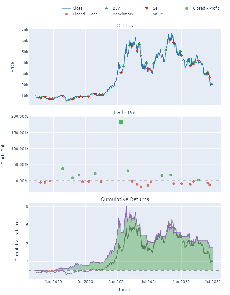
Here is the plot. It contains PnL for each trade.
 Backtrader might be a more realistic test for trading I think. While giving the same condition to Backtrader, some trades are failed to execute due to lacking enough money. Putting 100% of portfolio for each trade results in cancellation of order occasionally. I have to adjust the trading size of portfolio in order to mimic the trade results above.
The result from Backtrader is:
 And that’s it! I briefly work through these 3 methods for implementing a trading strategy. Hopefully this article provides some insights for your trading journey! Here is the link of the code if you feel like digging deeper. Also a video is provided for explaining the notebook.